Peeling Documentation

Peeling

Peeling is a methode to compute the likelihood for a pedigree, it also enable the calculation of genotype probabilities for each member of the pedigree. There is two main method of peeling: Recursive Algorithm and Iterative Algorithm both have they own benefit and drawback.

The main equation of Peeling method aim the The conditional probability that pedigree member \(i\) has genotype \(u_i\) given all the genotypic data \(y\)

\[ \textcolor{orange}{Pr(u_i|y)} = \frac{ \textcolor{red}{a_i(u_i)}\textcolor{green}{g(y_i|u_i)}\textcolor{blue}{\prod p_{ij}(u_i)}}{L} \]

To compute this probability we need to compute each part of the equation.

Anterior function

This; \(\textcolor{red}{a_i(u_i)}\) is the Anterior function. It compute the joint probability of phenotypes of members anterior to \(i\) and of genoype \(u_i\) for \(i\).

\[ \begin{align} \textcolor{red}{a_i(u_i)} =\sum_{u_m}\Bigg\{ \textcolor{red}{a_m(u_m)}\textcolor{green}{g(y_m|u_m)}\textcolor{blue}{\prod_{\stackrel{j\in S_m}{j\ne f}}p_{mj}(u_m)} \times \newline \sum_{u_f}\Bigg\{\textcolor{red}{a_f(u_f)}\textcolor{green}{g(y_f|u_f)}\textcolor{blue}{\prod_{\stackrel{j\in S_f}{j\ne m}}p_{fj}(u_f)}\times \textcolor{magenta}{tr(u_i|um,uf)} \times \\ \prod_{\stackrel{j\in C_mf}{j\ne i}}\Bigg[\sum_{u_j}\textcolor{magenta}{tr(u_j|u_m ,u_f)}\textcolor{green}{g(y_i|u_i)} \textcolor{blue}{\prod_{k \in S_i}p_{kj}(u_k)}\Bigg]\Bigg\}\Bigg\} \end{align} \]

Penetrance function

The Penetrance: \(\textcolor{green}{g(y_i|u_i)}\) is if the real genotype of \(i\) is \(u_i\) the probability to observe \(y_i\). Due to sequencing error \(\varepsilon\) there is a shift between observed data and real value. So we can compute this conditional probability simply using an error matrix:

\[ \left[ \begin{array}{c|ccc} \text{real } u_i \downarrow \; \backslash \; \text{observed } y_i \rightarrow & \text{AA} & \text{AB} & \text{BB} \\ \hline \text{AA} & (1-\varepsilon)^2 & 2\times(1-ε)ε & \varepsilon^2 \\ \text{AB} & 2\times(1-ε)ε& (1-\varepsilon)^2 + \varepsilon^2 & 2\times(1-ε)ε \\ \text{BB} & \varepsilon^2 & 2\times(1-ε)ε & (1-\varepsilon)^2\\ \end{array} \right] \]

In this matrix error rate is \(\varepsilon\) let’s take some example to explaine:

• If real genotype is AA observe data is also AA then genotyping succed 2 times in a row, and the probability of succes is \((1-\varepsilon)\) for each chromosome: \((1-\varepsilon)^2\)
• In a case of a real genotype BB but observed data is AB that’s mean the sequencing of the first chromosome is good but the second not and vise versa. So the probability to miss only one from two genotype is \((1-ε)ε\) therefore considering both case is: \(2\times(1-ε)ε\)

Posterior function

The Posterior function \(\textcolor{blue}{\prod p_{ij}(u_i)}\) gives the joint probability of genotype of pedigree members posterior to \(i\) through its mates \(j\) and also through its offsprings \(k\)

\[ \textcolor{blue}{p_{ij}(u_i)} = \sum_{u_j}\Bigg[\textcolor{red}{a_j(u_j)}\textcolor{green}{g(y_j|u_j)}\textcolor{blue}{\prod_{\stackrel{k\in S_j}{k\ne i}}p_{jk}(u_j)}\times \prod_{k\in C_{ij}}\Bigg[\sum_{u_k}\textcolor{magenta}{tr(u_k|u_i ,u_j)}\textcolor{green}{g(y_k|u_k)} \textcolor{blue}{\prod_{l \in S_k}p_{kl}(u_k)}\Bigg]\Bigg] \]

Transmisson function

The transmission function doesn’t apear directly in the peeling function, but is present in Anterior and Posterior functions as \(\textcolor{magenta}{tr(u_i|u_m ,u_f)}\).

Transmission function gives the probability to observe the genotype \(u_i\) giving the genotype of its mother \(u_m\) and its father \(u_f\). Like the Penetrance this function can be illustrate with a matrix, but in this case the matrix shape is \(3\times3\times3\) to consider the 3 possible genotypes for the 3 individual.

For exemple if we consider the individual’s genotype is AB then the transmission matrix is:

\[ \left[ \begin{array}{c|ccc} \text{} u_m \downarrow \; \backslash \; \text{ } u_f \rightarrow & \text{AA} & \text{AB} & \text{BB} \\ \hline \text{AA} & 0.0 & 0.5 & 1.0 \\ \text{AB} & 0.5 & 0.5 & 0.5 \\ \text{BB} & \textcolor{red}{1.0} & 0.5 & 0.0\\ \end{array} \right] \]

So the probability having a child AB giving a father AA and a mother BB is 100% (the red cell in the matrix above). In the equation we right it: \(\textcolor{magenta}{tr(AB|AA ,BB)} = 1.0\).

Recursive Algorithm

As you see above those functions refer to the other and sometimes itself. Recursive algorithms are perfect for this kind of jobs.

Benefit of using recursivity

Apply recursive algorithm enable to strictly apply the formula. therefore compute an exact result.

Main drawback

If the explored pedigee had loops then the algorithm is totally inefficient, due to its recursive aspect. Indeed adding an inbreeding in pedigree (which append a lot in selection) will break the algorithm. Because at some point you’ll need \(\textcolor{red}{a_i(u_i)}\) to calculate \(\textcolor{red}{a_i(u_i)}\) for exemple.

Iterative Algorithm

The main goal of iterative peeling is to overcome recursive algorithm’s problem. But the equation can’t be solve without getting through the pedigree recursivly. hopefully there is a trick

The trick

The Problem of interative peeling is, for example, to compute \(\textcolor{red}{a_i(u_i)}\) you need to know sevral things such as \(\textcolor{red}{a_m(u_m)}\). But at the begining you dont have any information about anterior, so the trick is to set all unknown data at 1 and calculate each individual generation by genration (from the oldest to the newest) this step is called Peeling up. It’s followed with a Peeling down operation where information from an individual’s ancestors is used to infer the individual’s genotypes and allele origins. Repeating these operations propagates genetic information between members of a pedigree.

Peeling down

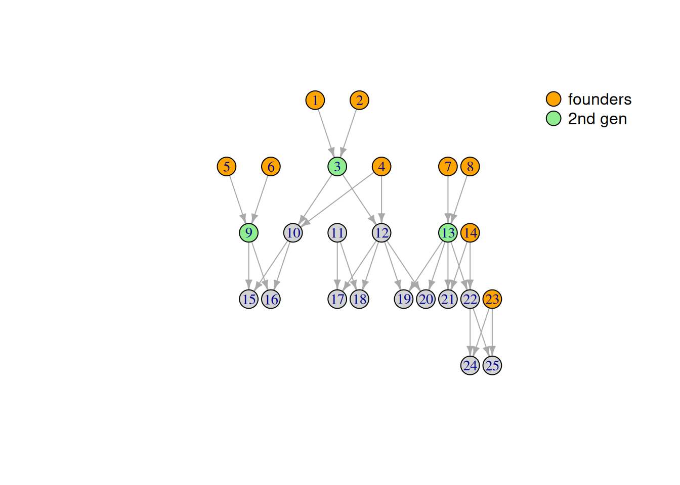
To perform a peeling down you need to indentifie generations. first generation called founders. and the second generation is individuals that both parents are founders. peeling down is the iterative calculation of each \(\textcolor{red}{anterior}\) throught generation, from the oldest to the youngest.

The \(\textcolor{red}{anterior}\) of a founders is simply the alelle frequency of founders. then to calculate 2nd generation’s \(\textcolor{red}{anterior}\) you need to know founder’s \(\textcolor{red}{anterior}\), \(\textcolor{green}{penetrance}\) and \(\textcolor{blue}{posterior}\). we don’t compute \(\textcolor{blue}{posterior}\) yet. but it initialise at \(1\).

Peeling UP

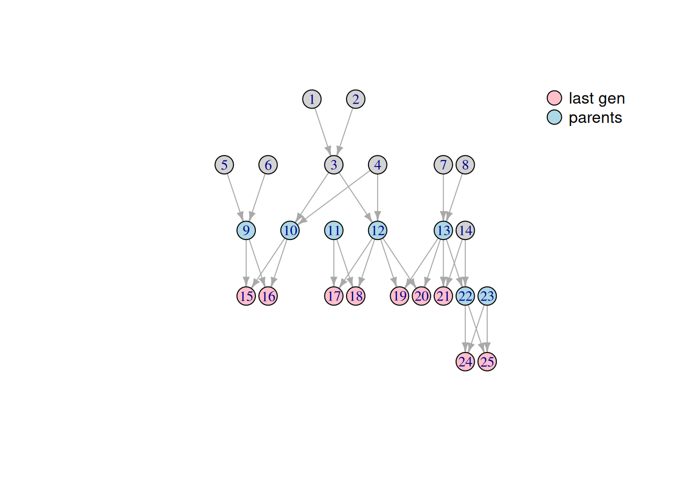
The Peeling Up prossess is to compute \(\textcolor{blue}{posterior}\) of ech individus. so we run \(\textcolor{blue}{posterior}\) calculation througth pedigrees, from the yougest to the oldest generation. The \(\textcolor{blue}{posterior}\) of the last generation is 1. Then we compute \(\textcolor{blue}{posterior}\) of they parents throught them.

Do this two operation peeling up an peeling down is called a cycle. Every cycle refine genetic information of individuals. To process an Iterative peeling, you run cycles until you get stable information up to 20 cycles.

Benefit of Iterative calculation

The iterative peeling enable to process peeling on pedigree with loops, pretty common in selection.

Drawback

Unlike the recursive one, iterative peeling approximate the genetic information. It cannot compute exact probability.

based on An efficient algorithm to compute the posterior genotypic distribution for every member of a pedigree without loops’s paper