Imputation of low-pass genotypes using pedigree-based methods

Compte rendu Stage M2

Lionel Viguier

1 Apr, 2026

Méthodes de génotypage

Genotype array

• Restricted number of loci
• Low error rate
• Low cost

Low-pass sequencing

• low coverage (<3X)
• Missing data
• Low cost

High coverage sequencing

• Exhaustive
• Expensive
• Low number of samples

Low-pass \(\rightarrow\) Requires imputation algorithms

• Il sacrifie la profondeur de séquencage (<5X) au profit du nombre de sample séquencé
• Il permet de garder l’information relative a l’individus
• Grace a un systeme d’imputation basé sur le LD il permet une amélioration de la confiance dans les données
• Permet d’obtenir une information sur le génome complet

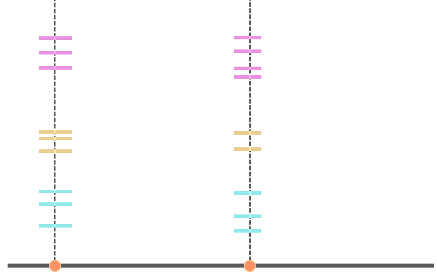
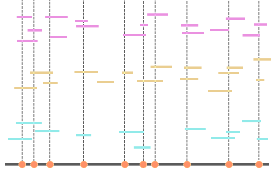
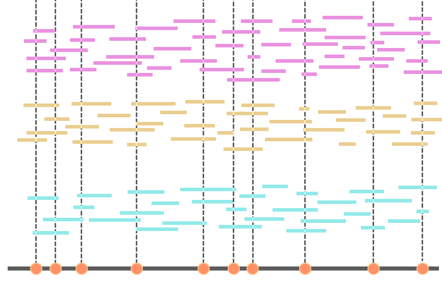
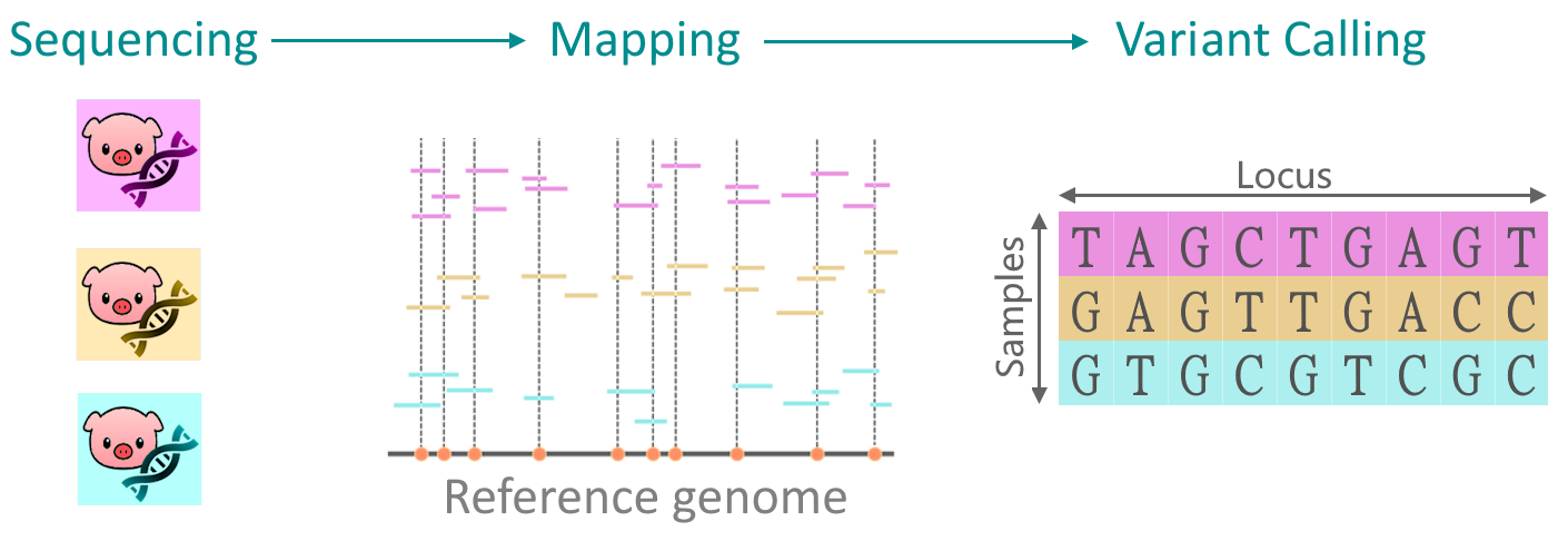
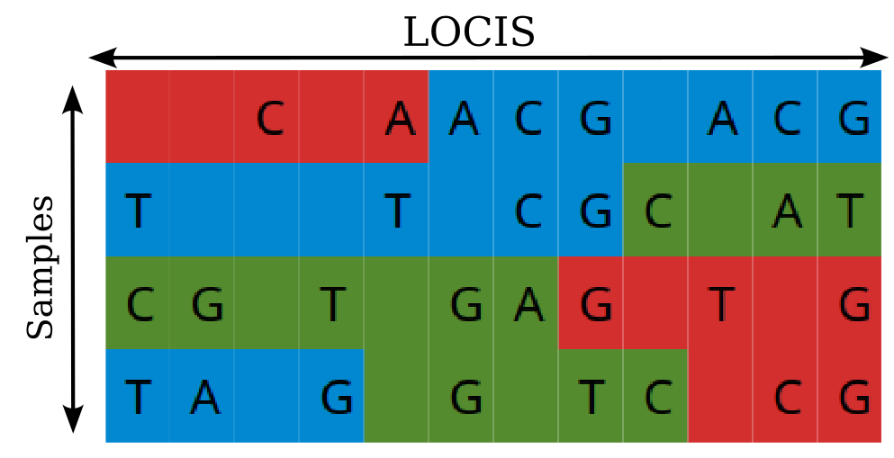
Du séquencage aux Variant Calling File (.vcf)

Vraisemblance de chaque génotypes

Penetrance: Distribution de la vraisemblance de chaque génotypes

Table 1: Probability distribution of individual \(i\) for \(u_i \in \{0,1,2\}\)

\(u_i\)	\(0\)	\(1\)	\(2\)
\(P(D|G)\)	0.01	0.23	0.81

Dans les fichiers de variant calling (.vcf)

Dans un .vcf on utilise le “Phredscore Likelihood” (PL)

\[ PL = -10 * \log{P(D | G)} \]

• Cette “confiance” dans les données peut s’exprimer comme \(P(D∣G)\) est appelé pénérance.
• La penetrance est la probabilitée conditionnelle que le vrais génotype d’un individu soit \(y_i\) sachant son génotypage
• c’est une distribution de densitée
• Dans un .vcf la penetrance ce présente sous forme de “Phredscore Likelihood” (PL)

Le \(_{raw}PL\) est normalisé \[ PL = _{raw}PL + max_{genotype}(_{raw}PL ) \]

Imputation

• Low-pass: Penetrance bruitée \(\rightarrow\) Imputation:
  • 2 méthodes existantes : LD-based et Pedigree-based (mendel)

Méthodes basées sur le LD

haplotypeTab

• Stitch (Davies et al. 2017)
• Glimpse (Rubinacci et al. 2021)

En low-pass la penetrance est très mauvaise car la profondeur de séquencage est très faible il est donc nésséssaire d’améliorer la qualité en faisant de l’imputation. Plusieurs approches existes

les deux méthodes se base sur le LD (déséquilibre de liaison)

essaie de créer une liste d’haplotype ancetres pour pouvoir identifier l’haplotype de chaque région pour chaque individus.

• Stitch (Davies et al. 2017)
  • sans Panel de référence
  • Il créer un panel d’haplotypes ancestrau pour associer chaque partie du génome a un haplotype
    
• Glimpse (Rubinacci et al. 2021)
  • Utilise Un panel de referance (séquencage 30X)
  • Se sert du Panel de référence pour pouvoir associer des haplotype a chaque partie du génome

Imputation

Méthodes basées sur le pedigree

Pedigree

Exemple pedigree

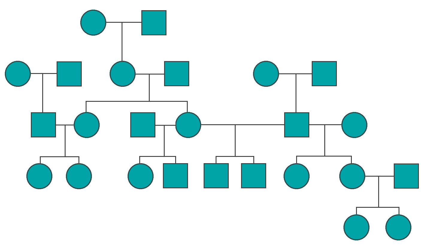
Exemples de méthodes

• FImpute
• Alphapeel

Imputation

Estimation de \(P(u_i|Y) \rightarrow\) Peeling

Fernando et al. 1993

Utilise les donnée phénotypiques et de pedigree des individus afin de calculer la probabilitée conditionelle des génotypes sachant les donnée phénotypique.

• Avec l’apparition du séquencage par puce cette méthode est devenu désuète.
• Retrouve un interet dans le contexte de séquencage low-pass.

Le Peeling permet de valoriser la mesure de Penetrance fournie par les approches low-pass

Peeling

Formule Fernando et al.

\[ \textcolor{orange}{Pr(u_i|y)} \propto \textcolor{red}{a_i(u_i)}\textcolor{green}{g(y_i|u_i)}\textcolor{blue}{\prod p_{ij}(u_i)} \]

Avec:

• \(\textcolor{green}{g(y_i|u_i)}\) ~ \(P(D|G)\)
• \(\textcolor{red}{a_i(u_i)} \rightarrow\) Anterior
• \(\textcolor{blue}{ p_{ij}(u_i)} \rightarrow\) Posterior

Peeling

Formule Fernando et al.

fonction Posterior

\[ \begin{align} \textcolor{blue}{p_{ij}(u_i)} = \sum_{u_j}\Bigg[\textcolor{red}{a_j(u_j)}\textcolor{green}{g(y_j|u_j)}\textcolor{blue}{\prod_{\stackrel{k\in S_j}{k\ne i}}p_{jk}(u_j)} \\ \times \prod_{k\in C_{ij}}\Bigg[\sum_{u_k}\textcolor{magenta}{tr(u_k|u_i ,u_j)}\textcolor{green}{g(y_k|u_k)} \textcolor{blue}{\prod_{l \in S_k}p_{kl}(u_k)}\Bigg]\Bigg] \end{align} \]

Peeling

Formule Fernando et al.

fonction Anterior

\[ \begin{align} \textcolor{red}{a_i(u_i)} =\sum_{u_m}\Bigg\{ \textcolor{red}{a_m(u_m)}\textcolor{green}{g(y_m|u_m)}\textcolor{blue}{\prod_{\stackrel{j\in S_m}{j\ne f}}p_{mj}(u_m)} \\ \times \sum_{u_f}\Big\{\textcolor{red}{a_f(u_f)}\textcolor{green}{g(y_f|u_f)}\textcolor{blue}{\prod_{\stackrel{j\in S_f}{j\ne m}}p_{fj}(u_f)}\\ \times \textcolor{magenta}{tr(u_i|u_m,u_f)} \\ \times \prod_{\stackrel{j\in C_mf}{j\ne i}}\Big[\sum_{u_j}\textcolor{magenta}{tr(u_j|u_m ,u_f)}\textcolor{green}{g(y_i|u_i)} \textcolor{blue}{\prod_{k \in S_i}p_{kj}(u_k)}\Big]\Big\}\Bigg\} \end{align} \]

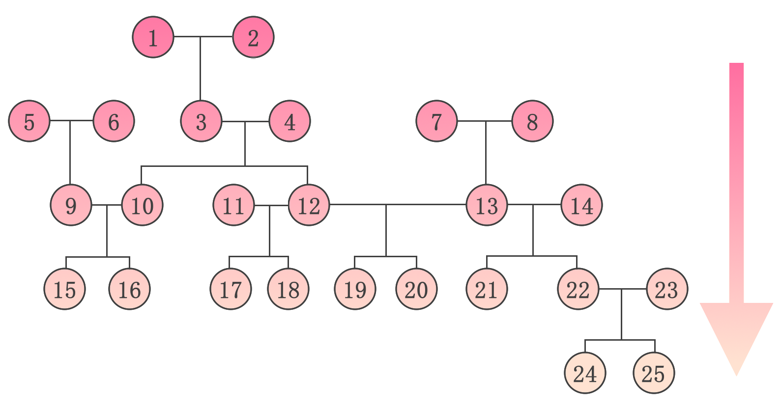
Peeling

Aspect récursif

• Récursivité : fonctions qui s’appellent elles-mêmes
• Conditions d’arrêts:
  • posterior: Individus sans enfants \(\rightarrow\) 1
  • anterior: Fondateurs \(\rightarrow\) \(\hat{f}\)

Inconvénient majeur

Exemple de pedigree avec boucle

Boucles récursivité impossible

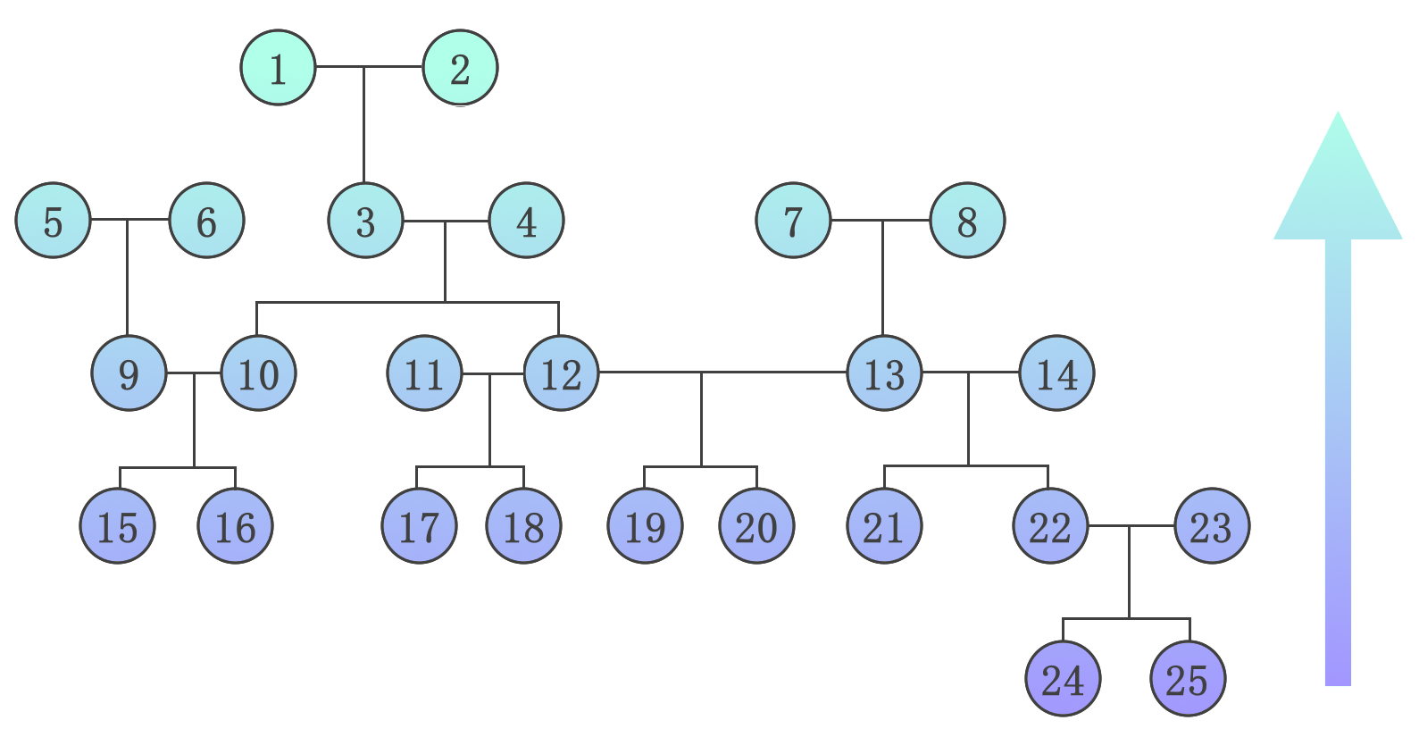
Iterative Peeling

• L’algorithme iteratif (Kerr et Kinghorn, 1996.)
  • pro: pedigree avec boucles
  • con: \(\widehat{P(u_i|Y)}\)

Fonctionnement

• Initialisation des antérieurs et posterieurs
• Repeat :
  • Peel down
    • mise à jours des anteriors
  • Peel up
    • mise à jours des posteriors

Peeling down

Iterative Peeling

• L’algorithme iteratif (Kerr et Kinghorn, 1996.)
  • pro: pedigree avec boucles
  • con: \(\widehat{P(u_i|Y)}\)

Fonctionnement

• Initialisation des antérieurs et posterieurs
• Repeat :
  • Peel down
    • mise à jours des anteriors
  • Peel up
    • mise à jours des posteriors

Peeling up

Implémentation

• Outil yapp
• Python
  • calcul scientifique scipy
  • gestion de fichiers .vcf panda
  • stockage de données zarr
• gestion de projet Git
• travail en log
• scaling
  • démonstration
  • implémentation

Données simulées pedigree + genotypes: SimuPOP

Jeux de données

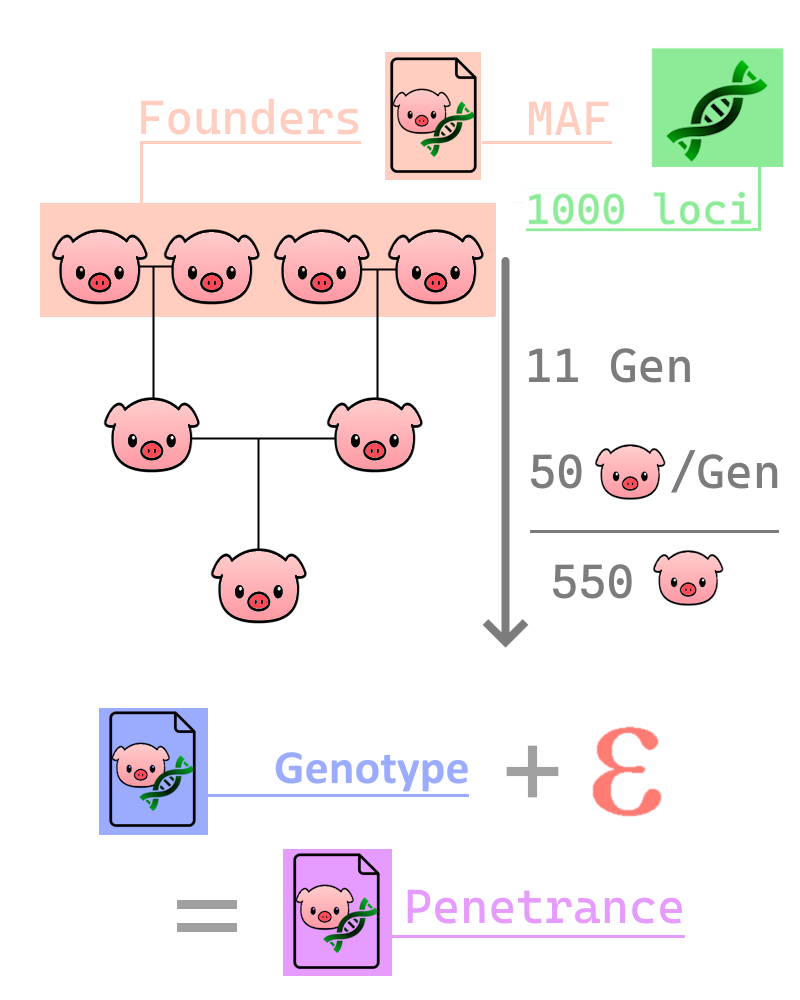
Simulation

• Génotype des fondateurs générés (algo coalescence)
• Générer un Pedigree (random mating)
• Génotype des individus générés
  • Transmission Mendélienne
  • loci indépendants
• Simulation de Penetrance Table 2

Table 2: For \(y_i=0\), i.e. AA

Observed \(y_i\)	Formula
0 (AA)	\((1-\epsilon)^2\)
1 (Aa)	\(2 \cdot (1-\epsilon) \cdot \epsilon\)
2 (aa)	\(\epsilon^2\)
NA	\(1\)

Problème numérique Scaling

• Problème: \(a_i(u_i)\) et \(p_{ij}(u_i)\) \(\simeq 0\)

• Solution:

Scaling: \[ \begin{cases} a_i(u_i)=C_i \centerdot a_i^* (u_i) \\ g_i(y_i|u_i)=E_i \centerdot g_i^*(y_i|u_i) \\ p_{ij}(u_i) = D_{ij} \centerdot p_{ij}^*(u_i) \end{cases} \]

• On a donc: \[ \textcolor{Tan}{Pr(u_i|y)}\propto a_i^* (u_i) g_i^*(y_i|u_i) \prod_j p_{ij}^*(u_i) \]

on scale anterior et posterior pour avoir \(valeur_{ui} - max_{u_i}(valeur_{ui})\)

pas besoin d’exponetier les valeurs

Test d’estimation de MAF

Taux d’erreur \(\epsilon = 10^{-4}\)

Taux d’erreur \(\epsilon = 10^{-1}\)

Qualité d’estimation (\(\epsilon = 10^{-1}\))

Distribution de densité (\(\epsilon = 10^{-1}\))

Simulation de données low-pass

Pour un tableau de génotypes connus \(G\) \((I,L)\)

Simuler \(P(Y = \{\textcolor{Emerald}{D},\textcolor{Apricot}{R}\}|G)\):

Pour chaque \(i,l\) avec \(l \in L\) loci et \(i \in I\) individus:

1. Tirer une profondeur \(\textcolor{Emerald}{D_{i,l}}\) où \(\textcolor{Emerald}{D_{i,l}} \sim \text{Poisson}(D_{\text{moy}})\)
2. Tirer \(\textcolor{Apricot}{R_{i,l}}\) reads où \(\textcolor{Apricot}{R_{i,l}} \sim \text{Binomial}(\textcolor{Emerald}{D_{i,l}},P = f(G_{i,l},\textcolor{BrickRed}{\epsilon}))\)
3. \(P(Y_{i,l} = \{\textcolor{Emerald}{D_{i,l}},\textcolor{Apricot}{R_{i,l}}\}|G_{i,l})= \begin{cases} 0: & \textcolor{BrickRed}{\epsilon}^{\textcolor{Apricot}{R_{i,l}}} \quad (1-\textcolor{BrickRed}{\epsilon})^{\textcolor{Emerald}{D_{i,l}} - \textcolor{Apricot}{R_{i,l}}} \\ 1: & \frac{1}{2}^\textcolor{Emerald}{D_{i,l}} \\ 2: & (1- \textcolor{BrickRed}{\epsilon})^{\textcolor{Apricot}{R_{i,l}}} \quad \textcolor{BrickRed}{\epsilon}^{\textcolor{Emerald}{D_{i,l}} - \textcolor{Apricot}{R_{i,l}}} \end{cases}\)
4. scaling

Table 3: probabilité d’observer un allele alternatif

\(G_{i,l}\)	\(0/0\)	\(0/1\)	\(1/1\)
\(f(G_{i,l},\textcolor{BrickRed}{\epsilon})\)	\(\textcolor{BrickRed}{\epsilon}\)	\(1\over2\)	\(1 - \textcolor{BrickRed}{\epsilon}\)

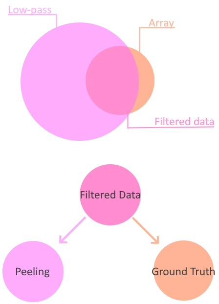
Données réelles (PorcQTL)

Donnée low-pass + array

• Évaluation sur Genotype array (Ground truth)
• \(P(u_i|Y)\) estimé sur du low-pass \(l \in L_{\text{array}} \cap L_{\text{low-pass}}\)

Données réelles : Ground truth (array) + Low-pass

Applications

Peeling avec des données low-pass:

• Imputation :
  • du génotype avec \(P(u_i|Y)\)
  • locus manquants
  • individus non génotypés
• Single-locus: \(\rightarrow\) besoin de méthodes utilisant LD

Assignation de parenté

Tester des parents candidats par rapport à un parent imputé

• Imputer le génotype du parent manquant
• Identifier le parent le plus probable

Perspectives du projet

• Test Genomewide
• Implémentation dans yapp
• Parallélisation
• Benchmark
  • Alphapeel
  • Glimpse
  • Stitch

Slide Bonus!

Le code potentiel de génération de Penetrance

from scipy import stats
import numpy as np
random_state = 43
N, L, Dm, epsilon = 10, 1000, 5, 0.01
G = np.random.choice((0,1,2), size = (L,N), replace=True)
D = stats.poisson.rvs(Dm,size = (L,N), random_state = random_state)
pf = np.array((epsilon,0.5,1-epsilon))
pf_G = pf[G.ravel()].reshape((L,N))
R1 = stats.binom.rvs(D,pf_G, random_state = random_state)
penetrance = np.stack([
    R1 * np.log(epsilon) + (D-R1) * np.log(1-epsilon),
    D*np.full((L,N),np.log(0.5)),
    R1*np.log(1-epsilon) + (D-R1) * np.log(epsilon)
],axis=-1)
penetrance = np.einsum("lnu->lun",penetrance)